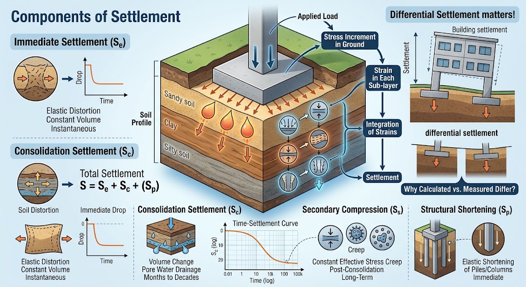
Foundation settlement analysis predicts how much a foundation will move downward under load, and how that movement develops over time. It combines an immediate response that occurs as the load is applied, a consolidation response that develops as pore water drains from fine-grained layers, and in some soils a long-term creep component.
Engineers perform this analysis because the serviceability of a structure is frequently governed by settlement rather than by bearing capacity. A foundation can be entirely safe against shear failure and still be unacceptable if it settles excessively, or if adjacent parts of the structure settle by different amounts.
The calculation follows a consistent sequence regardless of foundation type:
Applied load → Stress increment in the ground → Strain in each sub-layer → Integration of strains → Settlement
Each stage introduces its own assumptions, and the reliability of the result depends more on those assumptions than on the arithmetic that connects them.
What Are the Components of Foundation Settlement?
Total settlement is conventionally separated into components that develop through different mechanisms and over different time scales.
| Component | Symbol | Mechanism | Time scale |
|---|---|---|---|
| Immediate settlement | Se | Elastic distortion at constant volume | Effectively instantaneous |
| Consolidation settlement | Sc | Volume change as excess pore pressure dissipates | Months to decades |
| Secondary compression | Ss | Creep at constant effective stress | After primary consolidation |
| Structural shortening | Sp | Elastic shortening of piles or rigid columns | Immediate |
For a shallow foundation the total is:
S = Se + Sc
For a foundation on piles or rigid inclusions, the elastic shortening of the columns themselves is added:
S = Se + Sc + Sp
Settlement is not a single number. It is several mechanisms with different time scales, and a design decision usually depends on one of them rather than on their sum. Which mechanism governs, and the parameters behind it, are set out in the geotechnical report.
In cohesionless soils and unsaturated clays, immediate settlement generally predominates. In saturated cohesive soils, consolidation settlement becomes the predominant component; however, in highly organic soils, secondary compression or creep may be more significant.
How Is Immediate Settlement Calculated?
The immediate component is calculated by evaluating vertical strain at a series of depths and integrating it over the compressible zone.
Each soil layer defined in the soil profile is subdivided into a number of thinner sub-layers. This subdivision matters: stress increments decay rapidly with depth beneath a foundation, and a layer treated as a single unit will use a stress at its mid-height that does not represent its upper or lower portions.
At the mid-height of each sub-layer, the vertical strain is evaluated from the stress increments:
εᵢ = ( Δσz − 2ν · Δσh ) / Eᵢ
where Δσz is the vertical stress increment, Δσh the horizontal stress increment, ν Poisson’s ratio, and Eᵢ the deformation modulus of the layer to which the sub-layer belongs. Under the common assumption that horizontal stress increments are equal in both directions, and in undrained conditions where ν = 0.50, this expression reduces to the deviatoric stress increment divided by the modulus.
The compression of each sub-layer is then:
Se,ᵢ = εᵢ · hᵢ
and the immediate settlement at the point of interest is the sum over all sub-layers.
Which Modulus and Which Poisson’s Ratio?
This is where the drainage condition of the layer becomes decisive.
For layers analysed as undrained, the undrained modulus Eu and νu = 0.50 are used, and the calculated value represents settlement at constant volume immediately after loading. For layers analysed as drained, the effective modulus E′ and ν′ are used, and the calculated value represents the final settlement of that layer, since a freely draining layer does not develop significant excess pore pressure.
The same equation therefore produces a different physical quantity depending on the drainage assumption assigned to the layer. Selecting that assumption is an engineering decision, not a software setting.
Where Do the Stress Increments Come From?
Stress increments beneath a shallow foundation are obtained from elasticity theory, most commonly by integrating the Boussinesq point-load solution over the loaded area. For a foundation supported on piles or rigid columns, load is not applied at a surface but transferred into the ground along the shaft and at the base, and the Mindlin–Geddes solutions are used instead.
Where several foundations exist within one model, the stress increment at a given point is the sum of the contributions from all of them. This is what allows differential settlement between adjacent foundations to be evaluated rather than assumed.
A settlement calculation is only as deep as the compressible zone it was told to consider.
How Is Consolidation Settlement Calculated?
Consolidation settlement is calculated from one-dimensional consolidation theory, using the compression indices obtained from an oedometer test and the effective stress state of each sub-layer.
Three cases are distinguished, and the correct one depends on how the initial effective stress σ′₀ and the stress increment Δσ compare with the preconsolidation pressure σ′c.
Normally Consolidated Soil (σ′₀ = σ′c)
Sc = ( Cc · H / (1 + e₀) ) · log₁₀ ( (σ′₀ + Δσ) / σ′₀ )
Overconsolidated Soil, Loading Within the Recompression Range (σ′₀ + Δσ ≤ σ′c)
Sc = ( Cr · H / (1 + e₀) ) · log₁₀ ( (σ′₀ + Δσ) / σ′₀ )
Overconsolidated Soil, Loading Beyond the Preconsolidation Pressure (σ′₀ + Δσ > σ′c)
Sc = ( Cr · H / (1 + e₀) ) · log₁₀ ( σ′c / σ′₀ ) + ( Cc · H / (1 + e₀) ) · log₁₀ ( (σ′₀ + Δσ) / σ′c )
where Cc is the compression index, Cr the recompression index, e₀ the initial void ratio, and H the sub-layer thickness.
A fourth case exists for soils that have not completed consolidation under their own weight. These continue to settle regardless of the applied load, and settlement calculated from the structural load alone understates what the structure will experience.
Establishing σ′c for Each Sub-layer
The preconsolidation pressure is a property measured at a specific depth, but it must be applied to sub-layers throughout the thickness of a stratum. Applying a single laboratory value uniformly to a thick layer produces a preconsolidation profile that is physically inconsistent, because σ′c generally increases with depth in the same way that σ′v does.
A more defensible approach preserves the difference. The effective vertical stress σ′v is calculated at the depth from which the sample came, the difference (σ′c − σ′v) at that depth is established, and this difference is then added to the effective stress at the mid-height of each sub-layer:
σ′c,ᵢ = σ′v,ᵢ + (σ′c − σ′v) at sample depth
The overconsolidation ratio of each sub-layer follows:
OCRᵢ = σ′c,ᵢ / σ′v,ᵢ
Sub-layers with OCR greater than or equal to one are treated as overconsolidated, and those below one as normally consolidated. The equation applied to each sub-layer is then selected accordingly rather than being chosen once for the whole layer.
The consolidation equations rarely fail because the arithmetic is wrong. They fail because σ′c was assumed rather than established.
The parameters that feed these equations — Cc, Cr, e₀, σ′c — come from an oedometer test, and the procedures used to extract them from the test curves are discussed separately in the guide to the consolidation test.
Should Immediate and Consolidation Settlement Simply Be Added?
Not without consideration. Direct addition of undrained and consolidation settlement is a widely used convention, and EN 1997-1 Annex F notes explicitly that it can overestimate total settlement in many situations, so that empirical correction may be appropriate.
The reason is that the two calculations are not fully independent. The immediate calculation assumes distortion at constant volume, and the consolidation calculation assumes one-dimensional compression with lateral strain restricted. Real ground beneath a foundation of finite width does neither exactly, and the two idealisations overlap to some degree.
Adding the components is a convention, not a theorem.
In practice the convention is retained because it is transparent, conservative in most circumstances, and consistent with the way the parameters are measured. What it deserves is awareness rather than replacement: where predicted settlement is close to an acceptance limit, the magnitude of the overlap is worth examining before a design is changed on the basis of the sum.
How Is the Time–Settlement Curve Produced?
The magnitude of consolidation settlement answers only half of the question. The rate at which it develops is frequently the more important result, particularly where a structure is sensitive to movement occurring after it is put into service.
The rate follows from Terzaghi’s one-dimensional consolidation theory. For each layer, a dimensionless time factor is calculated:
Tv = cv · t / d²
where cv is the coefficient of consolidation, t the elapsed time, and d the length of the drainage path. The drainage path is the layer thickness divided by the number of drainage boundaries: a layer that can drain both upward and downward has d = H/2, while a layer draining in one direction only has d = H.
The degree of consolidation U is then read from the U–Tv relationship appropriate to the pore pressure distribution within the layer. Different distributions — uniform, linearly increasing, linearly decreasing — produce different U–Tv relationships, and the correct one depends on the boundary and drainage conditions of that particular layer.
Layer thickness + cv + drainage path → Tv → U → Sc(t)
The consolidation settlement realised at time t is the product of U and the final consolidation settlement of that layer. Summing across layers, and adding the immediate component, gives the total settlement at that time. Repeating the calculation over a series of times produces the time–settlement curve.
Where cv Comes From
The coefficient of consolidation is obtained from the oedometer test, using either the logarithm-of-time method to obtain t₅₀ or the square-root-of-time method to obtain t₉₀:
cv = Tv · d² / t with Tv = 0.197 at U = 50 % and Tv = 0.848 at U = 90 %
The two routes rarely give identical values. Which one is carried into the time–settlement analysis should be a deliberate choice rather than a default, because the difference propagates directly into predicted timescales.
The Construction Time Correction
Theoretical consolidation curves assume that the full load is applied instantaneously. No structure is loaded that way. Excavation removes load, construction reapplies it progressively over months, and consolidation begins during that period rather than after it.
Terzaghi’s correction addresses this by assuming that a load applied over a construction period tc can be treated as if it were applied instantaneously at tc/2. Settlement occurring during construction is taken as half of what instantaneous loading would produce at the corresponding time, and the curve after construction is shifted to the right by half the construction period.
The effect diminishes as time increases. For long-term predictions the correction changes little, but for movement expected within the first years of service it can change the answer materially.
Gross or Net Pressure: Which Should Be Used?
Settlement is driven by the change in stress, not by the total stress at foundation level. Where a foundation is placed in an excavation, the weight of the soil removed has already been carried by the ground, and reapplying only the difference is the physically correct treatment.
The net pressure is therefore:
qnet = q − γ · Df
Consolidation settlement should always be calculated from qnet, because the recompression of ground that has been unloaded and reloaded is precisely what the Cr branch of the consolidation equation represents. For the immediate component the choice depends on whether excavation heave is to be accounted for explicitly.
Using gross pressure where net is appropriate is one of the more common sources of overestimated settlement in deep basements, where γ·Df can represent a substantial fraction of the applied load. The corresponding treatment on the bearing capacity side is discussed in the guide to Terzaghi’s bearing capacity theory.
How Does Settlement Analysis Differ for Piles and Rigid Inclusions?
When load is carried by piles, micropiles, or ground improvement columns, the settlement calculation changes in two ways: the stress no longer enters the ground at foundation level, and the columns themselves compress.
Two approaches are used, and they answer slightly different questions.
Stress Transfer Below the Column Zone
The axial load is distributed among the columns, and the stress increment beneath toe level is calculated using the Mindlin–Geddes solutions, which account for load transferred along the shaft as well as at the base. Settlement is then evaluated for the sub-layers below the column zone in the same way as for a shallow foundation, and the elastic shortening of the columns Sp is added.
This approach is appropriate for structural piles, where the columns are stiff relative to the soil and carry a clearly defined share of the load.
The Equivalent Modulus Approach
For ground improvement columns, the improved zone is better represented as a composite medium. The soil profile is re-layered so that the improved zone becomes one or more layers with composite properties, and the composite modulus follows from the area ratio:
Ecom = ( n · Ac · Ec + ( A − n · Ac ) · Es ) / A
where A is the block area, n the number of columns, Ac the cross-sectional area of one column, Ec the column modulus, and Es the soil modulus. The derivation assumes equal vertical deformation of columns and surrounding soil.
Once the profile has been re-layered, the analysis proceeds exactly as for a shallow foundation, with Boussinesq stress increments applied through the composite layers. Related modelling considerations are discussed in pile foundation modelling.
Negative Skin Friction
Where columns pass through soft, compressible, or recently placed fill, the surrounding ground may settle more than the column. The soil then hangs on the column instead of supporting it, adding load rather than resisting it.
The additional load is transferred above the neutral plane — the depth at which column and soil move together — and produces settlement beyond that calculated from the structural load alone. This mechanism is only relevant where the surrounding soil is genuinely compressible; in stiff overconsolidated clays the relative movement required to mobilise it does not occur.
Why Does Calculated Settlement Differ From Measured Settlement?
Predicted and observed settlement rarely coincide exactly, and the reasons are usually traceable to a small number of recurring sources.
The deformation modulus is the most influential single input and the least precisely known. Values derived from correlations with field test data, such as those examined in SPT N value and friction angle relationships, carry scatter that propagates directly into the result.
The depth of the compressible zone determines how much ground contributes. Truncating the analysis too shallow removes real settlement from the calculation; extending it far below the influence of the foundation adds sub-layers whose contribution is negligible but which can obscure where the settlement is actually generated.
Sample disturbance affects consolidation parameters more than most other laboratory results. A disturbed sample typically produces a flatter compression curve, a less distinct break, and a σ′c that is underestimated — which moves sub-layers from the recompression branch to the virgin compression branch and overestimates settlement.
Above the groundwater table, calculated consolidation settlement generally exceeds what occurs, because the theory assumes a saturated soil in which volume change is governed by drainage of pore water.
Common Errors in Settlement Analysis
| Error | Consequence |
|---|---|
| Using gross pressure instead of qnet for consolidation | Settlement overestimated, sometimes substantially in deep basements |
| Treating a thick layer as a single sub-layer | Stress decay with depth not captured; result depends on where the mid-height happens to fall |
| Applying one σ′c throughout a stratum | Sub-layers assigned to the wrong branch of the consolidation equation |
| Mixing Eu with drained analysis, or E′ with undrained | The calculated quantity no longer corresponds to the intended time condition |
| Ignoring construction time in the time–settlement curve | Post-construction movement overstated |
| Using cv from t₅₀ and t₉₀ interchangeably | Predicted timescales differ without the difference being acknowledged |
| Evaluating settlement only at the foundation centre | Differential settlement, which usually governs, not evaluated at all |
The last of these deserves emphasis. Structures are rarely damaged by uniform settlement. They are damaged by differential settlement, which cannot be identified from a single calculation point.
Where SETAF2018 Fits
SETAF2018 calculates settlement using established analytical methods rather than a general finite element model, on the basis that most foundation settlement problems are well represented by elasticity theory combined with one-dimensional consolidation.
Settlement points are defined by coordinate anywhere in the model, and at each point the stress increments from all defined foundations are superposed. Because any number of points can be defined, differential settlement between and within foundations is evaluated directly rather than inferred.
Each layer is automatically subdivided into sub-layers, with the number set by the user during profile definition. Stress increments are calculated at each sub-layer mid-height using Boussinesq integration for shallow foundations and Mindlin–Geddes for rigid columns, in either Cartesian or cylindrical coordinates. Effective stress, σ′c and OCR are established per sub-layer using the difference method described above, and the appropriate consolidation equation is selected for each.
Time–settlement curves are produced from the time factor and the U–Tv relationship matched to the pore pressure distribution defined for each layer, with cv taken from either t₅₀ or t₉₀, and with Terzaghi’s construction time correction applied where a construction period is entered. Results are available as both tables and curves, and the underlying equations appear in the calculation reports rather than only the final values.
The derived settlement also feeds the vertical modulus of subgrade reaction used in structural models, which is one reason the settlement analysis and the spring stiffness handed to a structural engineer remain consistent with one another. Analysis, design checks, drawings, and reporting for shallow and deep foundations are carried out within the same model.
Where a problem genuinely requires modelling of interaction effects that these methods do not represent — strongly interacting foundation systems, or deformation-sensitive work adjacent to existing structures — the considerations involved in moving to a continuum model are discussed in the guide to finite element analysis in geotechnical engineering.
Frequently Asked Questions
What is foundation settlement analysis?
It is the calculation of how much a foundation will move downward under load and how that movement develops with time. The analysis combines an immediate elastic response, a consolidation response caused by drainage of pore water from fine-grained layers, and where relevant the elastic shortening of piles or columns.
What is the difference between immediate and consolidation settlement?
Immediate settlement occurs as the load is applied and involves distortion at constant volume, calculated using undrained parameters. Consolidation settlement develops over months or years as excess pore water pressure dissipates and the soil reduces in volume, calculated from the compression indices and the effective stress state.
How is consolidation settlement calculated?
From the compression index Cc, the recompression index Cr, the initial void ratio e₀, and the change in effective stress, using logarithmic expressions applied to each sub-layer. Which expression applies depends on whether the final effective stress remains below or passes above the preconsolidation pressure σ′c of that sub-layer.
How long does consolidation settlement take?
The duration is governed by the coefficient of consolidation cv, the thickness of the compressible layer, and the number of drainage boundaries. Because the time factor depends on the square of the drainage path, doubling the thickness of a layer increases the time to a given degree of consolidation approximately fourfold.
Should immediate and consolidation settlement be added together?
Direct addition is the usual convention and is generally conservative, but EN 1997-1 Annex F notes that it can overestimate total settlement, so that empirical correction may be appropriate. Where predicted settlement is close to an acceptance limit, the degree of overlap between the two idealisations is worth examining.
Which settlement matters more, total or differential?
Differential settlement usually governs. Structures accommodate uniform settlement comparatively well, whereas differential movement induces additional forces in the structure and is the more common cause of cracking and serviceability problems. Evaluating settlement at several points rather than one is what makes it visible.
Is finite element analysis required for settlement calculation?
Not for most foundation problems. Elasticity-based stress distribution combined with one-dimensional consolidation theory is well established, supported by design standards, and appropriate for the majority of routine settlement calculations. Advanced numerical modelling becomes valuable when interaction effects, unusual geometry, or strongly nonlinear behaviour govern the engineering question.
Why is calculated settlement often larger than what is measured on site?
Common causes include using gross rather than net pressure, sample disturbance that lowered the apparent preconsolidation pressure, a conservatively selected deformation modulus, adding immediate and consolidation components without considering their overlap, and applying saturated consolidation theory to layers above the groundwater table.