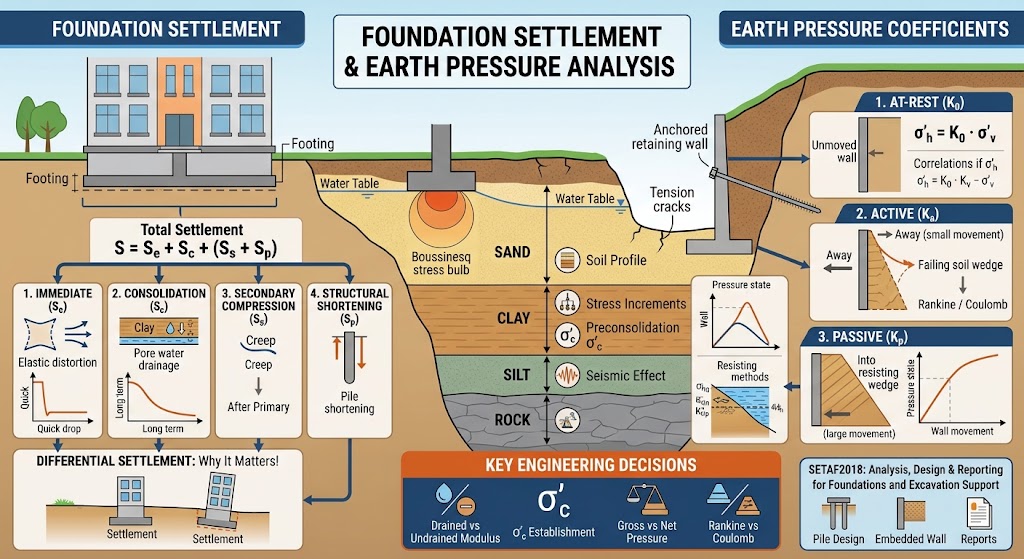
An earth pressure coefficient is the ratio between the horizontal effective stress acting on a wall and the vertical effective stress at the same depth. It converts a known vertical stress into the horizontal pressure that a retaining structure must resist, and its value depends on how far, and in which direction, the wall has moved.
Three states are distinguished. The at-rest coefficient K₀ applies when the wall has not moved. The active coefficient Ka applies when the wall has moved away from the soil far enough for the soil to reach failure while pushing. The passive coefficient Kp applies when the wall has moved into the soil far enough for the soil to reach failure while resisting.
Wall movement → Pressure state → Coefficient → Horizontal pressure
The most important consequence of that sequence is often overlooked in practice:
An earth pressure coefficient is not a property of the soil. It is a statement about how much the wall has moved.
What Are the Three Earth Pressure States?
| State | Coefficient | Wall movement | Relative magnitude |
|---|---|---|---|
| At-rest | K₀ | None | Intermediate |
| Active | Ka | Away from the retained soil | Lowest |
| Passive | Kp | Into the soil | Highest |
The horizontal effective stress in each state follows directly from the coefficient:
σ′h = K · σ′v
with water pressure added separately where a groundwater table is present, since water transmits pressure equally in all directions and is not scaled by an earth pressure coefficient.
For a soil with an effective friction angle of 30°, the three coefficients differ by roughly a factor of nine between active and passive. That range is why the assumed state matters more than small variations in the strength parameters used to compute it.
How Much Movement Is Needed to Reach the Active or Passive State?
The two limiting states are not reached at the same displacement, and this asymmetry governs how retaining structures actually behave.
The active state requires very little movement. A wall rotating away from the soil by a fraction of a percent of its height is generally sufficient to reduce pressures from at-rest to active in granular soils, with looser soils requiring somewhat more movement than dense ones.
The passive state requires considerably more — typically an order of magnitude greater displacement than the active state, and in some conditions more than that. This creates a practical difficulty. A wall that has moved enough to fully mobilise passive resistance in front of it may already have moved more than the structure it protects can tolerate.
Passive resistance is real, but it is not free. It has to be bought with displacement.
The design consequence is that full passive resistance is rarely available in a serviceability condition. This is one reason embedded wall analysis is normally carried out with a method that links pressure to displacement, rather than by assuming limiting pressures throughout.
How Is the At-Rest Coefficient K₀ Determined?
The at-rest coefficient describes the horizontal stress that exists in the ground before any wall is built or before it moves. It reflects the stress history of the deposit rather than a failure condition.
For normally consolidated soils, Jaky’s expression is the most widely used:
K₀ = 1 − sin φ′
For overconsolidated soils, the horizontal stress locked in during previous loading is retained after unloading, so K₀ increases with the overconsolidation ratio:
K₀ = ( 1 − sin φ′ ) · OCR^(sin φ′)
For fine-grained soils, correlations based on plasticity are also used, and the plasticity index enters the estimate in place of the friction angle.
K₀ is significant beyond its role in the initial stress state. It is the starting point for the pressure on an undeformed wall, it appears in the Chadeisson expression for the horizontal modulus of subgrade reaction, and in an overconsolidated clay it can exceed unity — meaning horizontal stress exceeds vertical stress, and a wall installed in such ground attracts more load than an at-rest coefficient below one would suggest.
Rankine Theory: What It Assumes and When It Applies
Rankine’s theory considers the state of stress in a semi-infinite soil mass at the point of failure, without reference to the wall itself. For a horizontal ground surface the coefficients reduce to their familiar form:
Ka = ( 1 − sin φ′ ) / ( 1 + sin φ′ ) = tan² ( 45° − φ′/2 )
Kp = ( 1 + sin φ′ ) / ( 1 − sin φ′ ) = tan² ( 45° + φ′/2 )
Where the ground surface behind the wall slopes at an angle β to the horizontal, the coefficients become:
Ka = cos β · ( cos β − √( cos²β − cos²φ′ ) ) / ( cos β + √( cos²β − cos²φ′ ) )
Kp = cos β · ( cos β + √( cos²β − cos²φ′ ) ) / ( cos β − √( cos²β − cos²φ′ ) )
Including cohesion, the horizontal pressures in an effective stress analysis are:
σ′a = Ka · σ′v − 2c′ · √Ka
σ′p = Kp · σ′v + 2c′ · √Kp
The cohesion term reduces active pressure and increases passive pressure. In the active case this produces a negative pressure near the surface, implying tension between soil and wall. Since soil cannot sustain tension against a wall, that portion of the diagram is normally set to zero, and the depth over which it occurs is treated as a tension crack that may fill with water.
The central assumption of Rankine’s theory is that there is no friction between the wall and the soil. That assumption has a direct consequence: because no shear can be transmitted at the interface, the resultant pressure must act parallel to the ground surface. For a vertical wall retaining level ground, this means a horizontal resultant.
Coulomb Theory: Adding Wall Friction and Geometry
Coulomb’s theory approaches the problem from equilibrium of a failure wedge rather than from the stress state of the soil mass, which allows it to include the geometry of the wall and the friction that develops along its back.
Four angles enter the calculation: the effective friction angle of the soil φ′, the inclination of the wall back from vertical α, the slope of the ground surface β, and the wall friction angle δ.
Ka = cos²(φ′ − α) / { cos²α · cos(α + δ) · ( 1 + √( sin(φ′ + δ) · sin(φ′ − β) / ( cos(α + δ) · cos(α − β) ) ) )² }
Kp = cos²(φ′ + α) / { cos²α · cos(α − δ) · ( 1 − √( sin(φ′ + δ) · sin(φ′ + β) / ( cos(α − δ) · cos(α − β) ) ) )² }
When the wall back is vertical (α = 0) and wall friction is neglected (δ = 0), these expressions reduce exactly to the Rankine coefficients. Coulomb’s theory contains Rankine’s as a special case rather than contradicting it.
Rankine and Coulomb do not disagree. They answer the same question with different amounts of information.
One well-known limitation deserves mention. The Coulomb passive coefficient assumes a planar failure surface, which becomes increasingly unrealistic as wall friction increases. For large values of δ the theory overestimates passive resistance, sometimes substantially. Where passive resistance governs and wall friction is high, methods based on curved failure surfaces give a more reliable answer.
Rankine or Coulomb: Which Should Be Used?
| Rankine | Coulomb | |
|---|---|---|
| Basis | Stress state in the soil mass | Equilibrium of a failure wedge |
| Wall friction δ | Not considered | Included |
| Inclined wall back | Not considered | Included |
| Sloping ground | Included | Included |
| Direction of resultant | Parallel to ground surface | Inclined by δ from the wall normal |
| Active pressure | Slightly conservative | Lower, generally closer to observed |
| Passive pressure | Conservative | Can be unsafe at high δ |
Neither is universally preferable. Rankine is simpler, transparent, and conservative for active pressure, which makes it a reasonable default where wall friction is uncertain or where a check calculation is wanted. Coulomb represents the physical problem more completely and generally produces more economical active pressures, at the cost of requiring a judgement about δ.
A defensible position adopted in much of practice is to use Coulomb for active pressure, where wall friction reduces the load and the planar surface assumption remains reasonable, while treating Coulomb passive values with caution where δ is large.
What Is the Wall Friction Angle δ?
The wall friction angle describes the shear resistance that develops along the interface between the soil and the back of the wall. Its physical origin is straightforward: as the soil wedge moves downward relative to the wall, friction along the contact carries part of the load, reducing the horizontal component that the wall must resist.
Its value depends on the roughness of the wall surface, the soil type, and the direction of relative movement. It is normally expressed as a fraction of the effective friction angle of the soil, with smoother interfaces and softer soils taking lower values.
Two points are worth keeping in view. First, δ affects the direction of the resultant as well as its magnitude — a wall analysed with wall friction receives an inclined thrust, which introduces a vertical component that must be accounted for in stability checks. Second, wall friction that acts favourably in the active case may not be reliably present in every condition, particularly where the wall settles relative to the soil rather than the reverse, which can reverse the sign of the interface shear.
How Are Earth Pressures Calculated in a Total Stress Analysis?
In fine-grained soils under short-term loading, pore water pressure has not had time to dissipate, and the analysis is carried out in total stress using undrained shear strength cu rather than effective parameters.
The coefficient in this case is not a ratio of stresses but an additive term:
Ku = 2 · √( 1 + a / cu )
where a is the adhesion between soil and wall, commonly taken as a fraction of cu. The horizontal pressures follow as:
σa = σv − Ku · cu
σp = σv + Ku · cu
Two differences from the effective stress case matter in practice. The undrained shear strength subtracts a constant from the vertical total stress rather than scaling it, which produces a very different pressure diagram shape. And the calculated active pressure can be negative over a substantial depth in a stiff clay, which again implies tension and requires the same treatment as the cohesion term in the effective stress case.
Whether the short-term or long-term condition governs depends on the soil and on the duration of the temporary works. In soft clays the undrained condition is usually more critical for stability; in stiff clays the long-term drained condition typically governs, because pore pressures that were initially negative equalise over time and pressures increase.
How Do Surcharge Loads Change the Pressure Diagram?
Loads applied to the ground behind a wall — traffic, stockpiles, crane outriggers, adjacent foundations — produce additional horizontal stress at the soil–wall interface.
These are not handled by scaling with an earth pressure coefficient. The horizontal stress increment is calculated from elasticity theory, by integrating the Boussinesq solution over the geometry of the load, and is then added to the active, passive, and at-rest pressures already computed.
Four load geometries cover most practical cases:
| Load type | Definition | Typical source |
|---|---|---|
| Point | A single concentrated force | Crane outrigger, column foundation |
| Line | Infinite length parallel to the wall, load per unit length | Strip footing, wall footing |
| Strip | Finite width, infinite length parallel to the wall | Road, railway, haul route |
| Area | Finite width and length | Stockpile, building footprint |
The distance from the wall governs the result strongly. A surcharge placed close to the wall produces a concentrated increase in pressure over the upper portion; the same load placed further back spreads its influence over a greater depth and reduces the peak.
Why Design Pressures Are Rarely Purely Active or Purely Passive
The three coefficients describe limiting conditions. A real embedded wall exists between them.
A wall that has deflected enough to reach the active state near mid-height may still be close to at-rest at the toe, where it is restrained, and nowhere near full passive on the excavation side. Assigning a single limiting state to the whole wall therefore misrepresents both the pressures and the structural forces that follow from them.
This is the reasoning behind analysis methods that treat pressure as a function of displacement. The ground is represented as an elasto-plastic spring: pressure begins at the at-rest value on the undeformed wall, migrates toward the active state where the wall moves away and toward the passive state where it moves in, and is bounded at those limits so that it can never pass beyond a physically achievable value.
At-rest (K₀) → wall deflects → pressure migrates toward Ka or Kp → bounded at the limiting value
The coefficients discussed in this article are therefore not replaced by such a method. They define the bounds within which it operates, which is why their determination remains consequential even when the analysis itself is numerical. How that framework is implemented, and how the spring stiffness within it is established, is discussed in the guide to the modulus of subgrade reaction and in the shoring system design guide.
Under seismic loading the same bounds shift: active pressure increases and passive resistance decreases as inertia acts on the soil wedge. That case is treated separately.
Common Errors in Earth Pressure Calculation
| Error | Consequence |
|---|---|
| Applying an earth pressure coefficient to water pressure | Water pressure underestimated; it acts equally in all directions and is not scaled by K |
| Assuming full passive resistance in a serviceability check | Resistance credited that the wall has not moved enough to mobilise |
| Using Coulomb passive with a high wall friction angle | Passive resistance overestimated because the planar failure surface assumption breaks down |
| Retaining the negative portion of the active diagram | Tension credited between soil and wall that cannot exist |
| Using K₀ = 1 − sin φ′ in a heavily overconsolidated clay | Horizontal stress substantially underestimated |
| Mixing effective and total stress parameters in one diagram | The resulting pressure corresponds to no physical condition |
| Placing a surcharge in the model without its actual distance from the wall | Peak pressure and its depth both misplaced |
The recurring theme is that each coefficient carries an assumption about wall movement, drainage condition, and interface behaviour. Transferring a number without its assumptions is what produces the error.
Where SETAF2018 Fits
SETAF2018 calculates at-rest, active, and passive pressures for every defined construction stage, both behind and in front of the wall, and uses them as the bounds within which the wall analysis operates.
Coefficients can be derived by Rankine or Coulomb theory, selected in the analysis settings, using the ground slope, wall back inclination, and wall friction angle δ defined for the section. K₀ is either entered directly or calculated from the effective friction angle and overconsolidation ratio of each layer as defined in the soil profile. Where a layer is analysed in total stress, the undrained coefficient and adhesion are used instead, and the pressure diagram is constructed accordingly.
Surcharge loads are defined as point, line, strip, or area loads with their actual geometry and distance from the wall, and their horizontal stress increments are obtained by numerical integration of the Boussinesq solution and added to the computed pressures. Loads can be designated permanent or variable so that partial factors are applied correctly.
Because the analysis follows the dependent pressures method, the coefficients are not applied as fixed diagrams. They establish the limits, and the pressure actually acting at each node follows from the calculated displacement at that node. The pressure diagrams, the coefficients used to produce them, and the equations behind both appear in the calculation reports, which allows a reviewer to confirm which theory and which parameters produced a given diagram rather than only seeing the result. The same framework applies across bored pile, diaphragm, sheet pile, and reinforced concrete wall types within excavation support analysis.
Frequently Asked Questions
What is an earth pressure coefficient?
It is the ratio of horizontal effective stress to vertical effective stress at a point in the ground. Multiplying the vertical effective stress by the coefficient gives the horizontal pressure acting on a retaining structure, with water pressure added separately.
What is the difference between Ka, Kp and K0?
K₀ applies to ground that has not moved and reflects the stress history of the deposit. Ka applies after the wall has moved away from the soil sufficiently for the soil to reach failure, and gives the lowest pressure. Kp applies after the wall has moved into the soil, and gives the highest pressure.
What is the formula for Ka and Kp?
For a vertical wall retaining level ground with no wall friction, Ka = tan²(45° − φ′/2) and Kp = tan²(45° + φ′/2). Where the ground slopes, the wall back is inclined, or wall friction is included, the Rankine or Coulomb expressions given above apply.
Which is better, Rankine or Coulomb?
Neither is universally better. Rankine is simpler and conservative for active pressure and requires no assumption about wall friction. Coulomb includes wall friction and wall geometry and generally gives more economical active pressures, but its passive coefficient becomes unsafe at high wall friction angles because it assumes a planar failure surface.
What is the wall friction angle δ?
It is the friction that develops between the soil and the back of the wall as the soil wedge moves relative to it. It is normally taken as a fraction of the effective friction angle of the soil, depending on wall roughness and soil type, and it reduces the horizontal component of active thrust while introducing a vertical component.
Why can active earth pressure be negative near the surface?
The cohesion term in the active pressure equation subtracts a constant from the pressure, and near the surface this can exceed the pressure produced by the vertical stress. Since soil cannot sustain tension against a wall, that part of the diagram is set to zero and the affected depth is treated as a tension crack.
How much wall movement is needed to reach the passive state?
Considerably more than for the active state — typically an order of magnitude greater. This is why full passive resistance is often unavailable within serviceability displacement limits, and why analysis methods that link pressure to displacement give a more realistic result than assuming limiting pressures.
Does K0 change with depth?
The coefficient itself is a property of the soil and its stress history rather than of depth, so it is constant within a layer of uniform properties. The horizontal stress it produces increases with depth because the vertical effective stress does. Where overconsolidation ratio decreases with depth, as it commonly does, K₀ decreases correspondingly between layers.